Do androids grow electric plants?

⚠️ Warning! This post is in a unfinished draft state. Placeholder sketches appear instead of interactive simulations. ⚠️

Animation commissioned by the band NIHILS.

Computation is a fundamental ingredient of the universe. Like atoms, quarks, gravity, electricity, the sun and moon, god and satan, death and taxes, computation is part of our cosmological story. Rather than simply being an occasional feature of natural processes, I believe natural processes can be understood as being computational at their very core.

In my art practice under the name SPACEFILLER (along with close collaborators), I attempt to express the computational beauty of nature¹ by “growing gardens” of lo-fi simulated plants. In this post, I will give an overview of the techniques I use to make these plants and explain more about my motivation for making them.

Rather than a step-by-step coding tutorial, this is a high level summary that will hopefully spark interest in technical and non-technical folks alike.

Frames divide time into discrete steps

You are probably familiar with the fact that a movie is composed of frames and that rapid playback of movie frames create the illusion of motion. If you play computer games, you might understand that they are composed of frames too. The computer refreshes your computer screen at some frequent interval (60 times a second, for example), and your eye perceives smooth motion constructed from a sequence of still images. In order to generate each frame, the computer must calculate the positions of objects within a scene and render those objects to the screen.

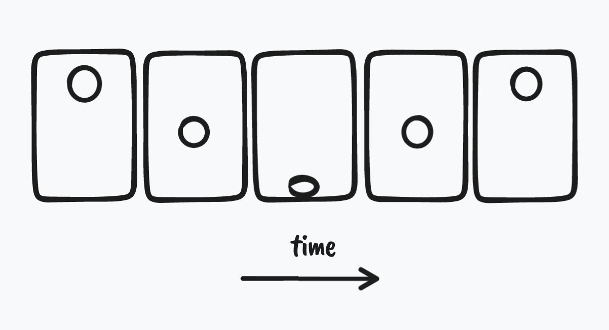
My plant simulation is no different. The configuration of plants is computed 60 times a second (or slower, depending on how large the simulation is). Furthermore, as is common for many simulations, each new frame’s state depends on the immediately previous frame’s state. This style of simulation is useful for mimicking the dynamics of the real world, because after all, the current state of the real world always depends on the previous state of the real world.²

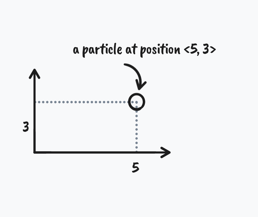
Particles divide stuff into discrete pieces

If frames are the fundamental unit of time of the plant simulation, particles are the fundamental unit of stuff. A particle represents a little piece of plant that can interact with other little pieces of plant. Each particle has a position (where the particle exists in 2D space) and velocity (the speed and direction the particle is moving in 2D space) which are represented as vectors.

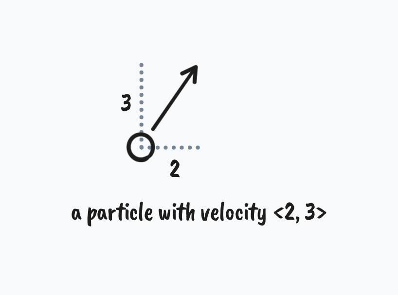
The behavior and interactions between particles are expressed as vector manipulations. (Vector math is out of the scope of this article, but I refer you to Daniel Shiffman’s excellent chapter on vectors in his book The Nature of Code.)

A symphony of forces

How do we control the motion of the particles? The answer is forces. We can apply a force to a particle to change its velocity, thereby creating motion. We make the simplifying assumption that all particles have the same mass, so applying a force to a particle looks like:

next velocity = previous velocity + force

In English, applying a force to a particle consists of adding a force vector to the velocity vector. A velocity’s next state depends on its previous state and the forces currently being applied to it. Multiple forces can be added simultaneously to a particle, pushing or pulling it in different directions. I have found that competing forces tend to result in interesting emergent behavior.

Now it is a matter of orchestrating a symphony of forces that push and pull particles into interesting forms and behaviors.

The base/bass: repulsive force

The base force of our system is the repulsive force. This drives particles away from each other if they are too close. The repulsive force provides order to the system. In the simulation below, compare the particles moving with random positions and velocities versus the particles with a repulsive force applied.

How do we compute the repulsive force? For each pair of particles, we find the distance between them:

If the distance is below a specified threshold, than we apply a force to each particle pointing away from the other particle:

The magnitude of the repulsive force depends on the inverse of the distance between particles. In other words, a larger force is applied if the particles are close together than if they are far part.

The repulsive force gives particles presence and weight. It allows particles to touch each other and exert influence on their particulate world. The repulsive force is like the bass guitar in a rock band, providing basic structure and organization to the whole affair that subsequent forces can build on top of.

Spring forces make shapes

That brings us to the next force in our symphony — the spring force. A spring force is a tad more complicated than a repulsive force because while a repulsive force only pushes particles away from each other, a spring force either pushes or pulls depending on the distance between particles.

A spring connects two particles together. Each spring has a spring length, and the spring force attempts to enforce this distance between connected particles. If the particles are too close (less than the spring length), a repulsive force is applied to push them apart. If the particles are too far (greater than the spring length), than an attractive force is applied to pull them together.

With springs in hand, we can bind particles together into interesting shapes.

Friction force

There has been a hidden force at work in the simulation that I haven’t mentioned yet: friction. Why do we need this?

One thing you quickly encounter with a particle system is that the particles are too energetic. That’s because by default, the particles live in a frictionless environment. Due to numerical errors that accumulate in a particle simulation, the lack of friction leads to runaway particles that move too fast.

TODO: example simulation

In the real world, objects exist in a thick fluid like air or water that stops them from moving too fast. Likewise, we need a healthy dose of friction to tame our wild particles.

The friction force always works opposite to a particle’s velocity:

TODO

It’s actually a very simple force to compute. All we need to do is multiply a particle’s velocity by a number less than 1 every timestep:

next velocity = friction * previous velocity

The lower the coefficient of friction, the more sluggish the particles.

TODO: example

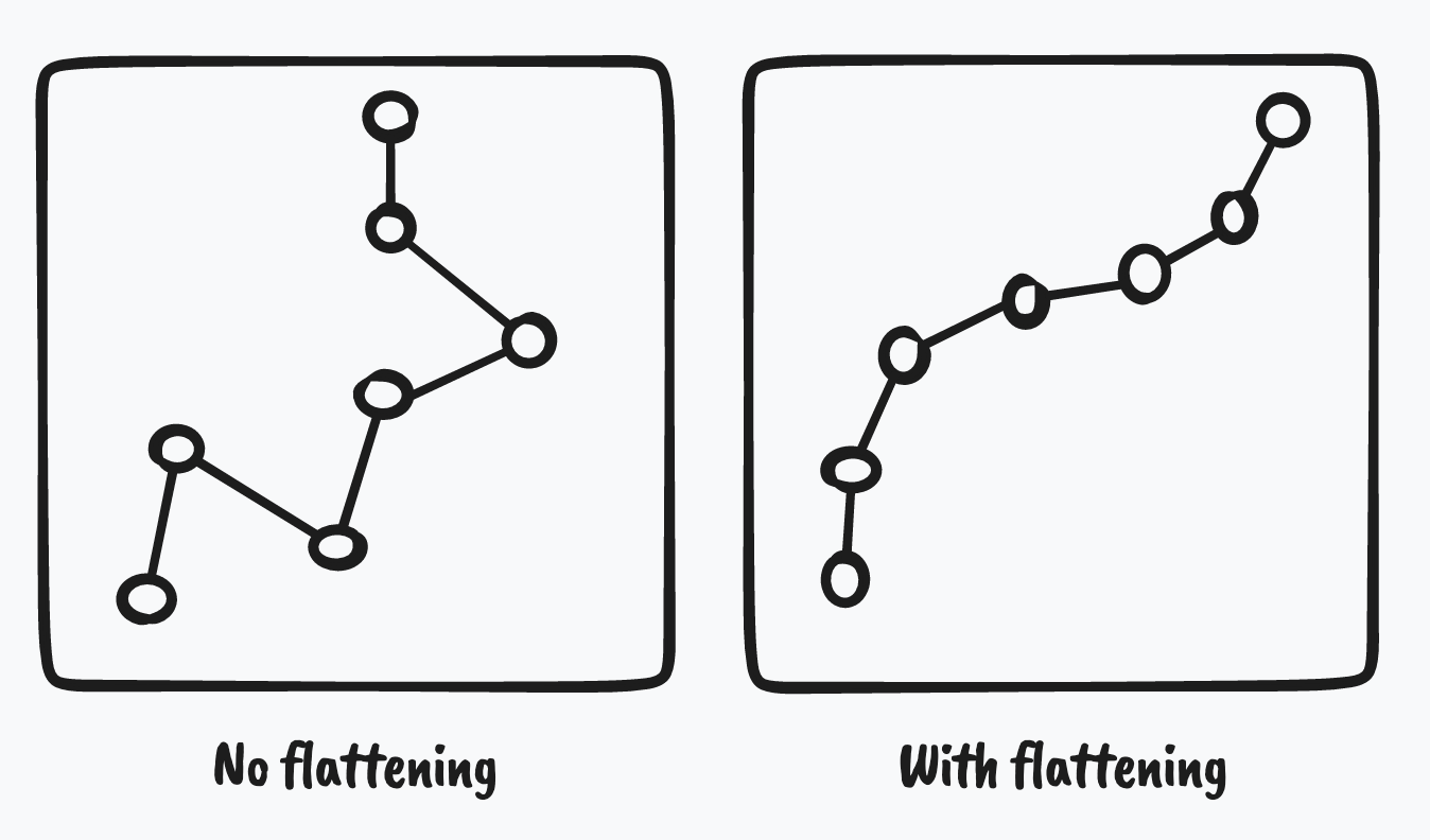
Flattening force

Connecting particles with springs allows you to design shapes, but a problem you quickly encounter is that chains of springs are zigzaggy rather than smooth. In order to achieve a smooth, organic look, a flattening force can be applied to particles in the chain.

To compute the flattening force:

1. Find the average position of spring-connected neighbor particles.
2. Apply a force in the direction of that average position.

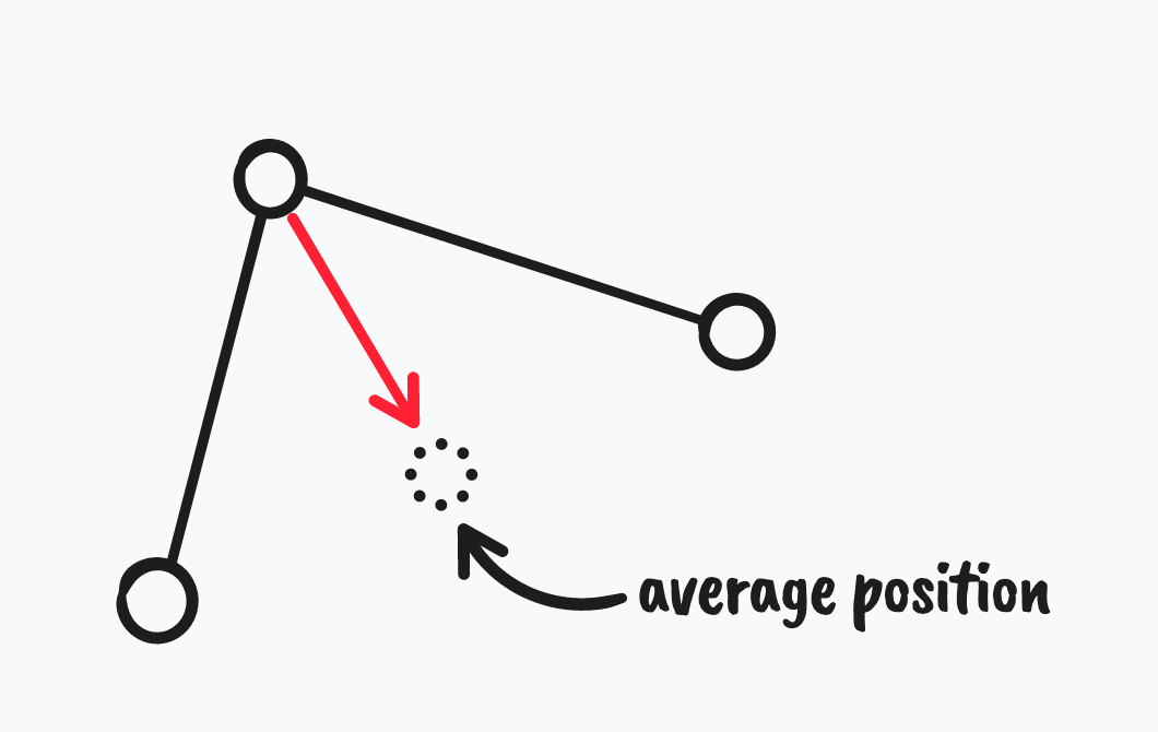
Moving towards the average position of spring-connected neighbors has the effect of reducing zigzag. The flattening force is like the supporting background vocals of a song: subtle when it is there, obvious when it is missing.

Birds of a feather

Thus far, our forces have been relatively “dumb”. They depend exclusively on the relative position of nearby particles (or, in the case of the friction force, they don’t depend on nearby particles at all). Consider what sort of behaviors would be possible if a force depended not only on nearby particle positions, but also on nearby particle velocities.

Imagine that you are going on a bike ride with a friend in their neighborhood (a neighborhood that you are not familiar with). Your first priority in steering your bike is to stay a certain distance away from your friend to avoid colliding with them. But at the same time, you must pay attention to where your friend is going, so that you can follow them. In other words, you observe their velocity, and steer / pedal to match their velocity (both direction and magnitude). If they steer right, you steer right. If they slow down, you slow down. And so on.

This velocity matching behavior is a tad more sophisticated than a simple push or pull force, and the resulting motion is more interesting. In Craig Reynold’s 1986 Boids algorithm, he applies this velocity matching concept to simulate bird flocking. His algorithm applies three constraints to each particle:

1. Separation
2. Cohesion
3. Alignment

TODO: Explain these & add pictures

For more information on steering behaviors and flocking, I again recommend Daniel Shiffman’s Nature of Code.

In my plant simulation, I sprinkled in some flocking creatures that live among the plants. I imagine that these are pollinating bees (although they look nothing like bees). They pluck flowers from plants and bring them back to their hives (this is also not a thing that bees do, but it seemed fun).

Todo:

• growth
  • particle chains
  • branching
  • inserting springs
• constraints
  • boxes
  • circles
  • SDFs
• optimization
  • spatial hashing
  • threads
  • quad tree
  • gpu
• architecture
  • particle system vs. simulation entities
  • tags

Artworks

TODO

In 2018 I was commissioned to build a permanent installation at an apartment building in Seattle, WA. I created a digital plant simulation which I called a Living Wall. Here is a clip of that installation:

I also recently released a series of algorithmically generated posters using the same underlying plant simulation.